Appendix A: Worked Tutorial Bank

A.1 Ride-Hailing

Environment:

traffic lights, travel times, traffic jams, charging-station occupancy

Resources:

fleet, vehicle types, capacities

Demand:

pickup, destination, time, passenger count, special needs

Exam use:

Separate the information model from the decision model. Demand and travel-time predictions are information. Acceptance, assignment, and repositioning are decisions.

Expanded worked model

Decision point:

whenever a request arrives, or every short planning interval

State \(S_k\):

time of day, vehicle locations, vehicle capacities/battery, open requests, traffic condition, charging-station availability

Decision \(x\in X(S_k)\):

accept/reject request, assign a vehicle, reposition idle vehicles, send a vehicle to charge

Post-decision state \(S_k^x\):

vehicle commitments and positions after assignment/repositioning, before the next request or travel-time realization

Stochastic information \(\omega_{k+1}\):

new requests, cancellations, travel-time realizations, charging-station occupancy

Spatial demand pattern example

Time	Typical origin density	Typical destination density	Operational implication
Morning	suburbs	downtown	preserve vehicles near residential pickup zones early
Evening	downtown	suburbs	reposition toward downtown before evening peak
Night	entertainment zones	mixed	value flexible nearby capacity

Exam answer pattern:

The ride-hailing problem is stochastic because future requests and travel times are unknown. It is dynamic because every assignment changes future vehicle availability and future service quality.

A.2 Service-Time Distribution

Model answer:

A service-time density is nonnegative, often right-skewed, and characterized by central tendency and spread. Rare long services can create scheduling risk.

Worked buffer calculation

Suppose service time \(T\) has:

Time	Probability
20	0.5
40	0.3
100	0.2

Expected time:

\[ E[T]=0.5\cdot20+0.3\cdot40+0.2\cdot100=42. \]

If the next appointment starts after 45 minutes:

\[ P(T>45)=0.2. \]

Business interpretation:

The average alone is not enough. The long tail creates a 20 percent risk of being late.

A.3 Pizza Delivery State

Tutorial state:

current time
status of three delivery drivers
information on customers yet to be served

Expanded state:

\[ S_k=(\text{time},\ \text{driver routes/availability},\ \text{open orders}, \ \text{locations},\ \text{order times},\ \text{travel-time information}) \]

Full MDP answer

MDP element	Pizza delivery answer
Decision point	each new order, each dispatch opportunity, or every few minutes
State \(S_k\)	current time, three driver statuses, current routes, open orders, locations, order times
Decision \(x\)	dispatch now or wait; assign orders to drivers; update routes
Cost \(R(S_k,x)\)	delay, travel time, lateness penalty, service-quality penalty
Post-decision state \(S_k^x\)	routes and driver availability after dispatch decision
Stochastic information \(\omega_{k+1}\)	new orders, prep completion, travel-time realization
Objective	minimize expected total delay/cost

Common mistake:

Do not put future unknown pizza orders into \(S_k\). Future orders are \(\omega_{k+1}\).

A.4 Trucks & Barges

MDP:

Decision points: each day
State: day, yard containers, destinations, due dates, known future containers
Decision: truck, barge, train, or hold
Cost: transport, setup, lateness, clean-up
Post-decision state: yard after shipments
Stochastic information: random arrivals and clean-up costs
Objective: minimize expected total cost

Policy Function Approximation rule design

The tutorial describes PFA implementation through filters, rules, and conditions. A business-friendly PFA can be written as:

If container is urgent and barge is not soon available, use truck.
If many containers share a destination and barge departure is soon, use barge.
If due date is far away and yard capacity is not tight, hold.

Formal policy:

\[ \pi_\theta(S_k)=x, \]

where \(\theta\) contains thresholds such as urgency cutoff, minimum barge fill, or maximum holding days.

Worked rule comparison

Rule	Merit	Risk
ship urgent containers by truck	avoids delay penalties	expensive if overused
consolidate non-urgent containers by barge	lowers unit cost	may miss deadlines
hold low-priority containers	preserves cheap transport option	increases yard congestion

Exam phrase:

A PFA is suitable when the policy can be expressed as operational rules using filters and conditions. It is fast and interpretable, but it may fail if thresholds are poorly tuned.

A.5 Dynamic Knapsack

State:

time, remaining capacity, current item

Decision:

accept or reject

PFA:

accept if Money / Space > threshold

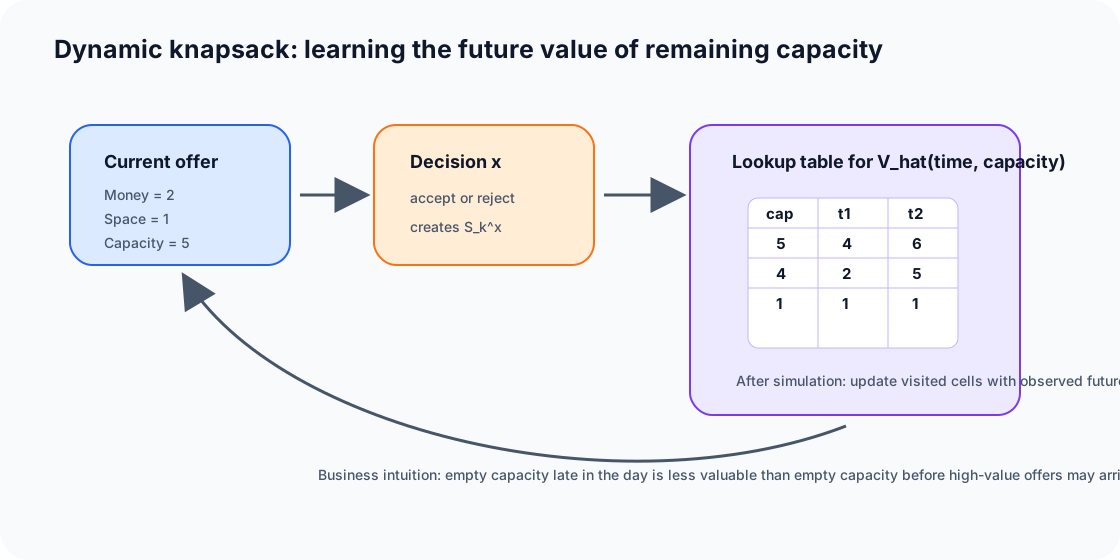
VFA insight:

Accepting a low-value item may be bad if it consumes capacity needed for future high-value items.

PFA threshold example

Accept if Money / Space > 1.

Offer	Money	Space	Ratio	PFA decision
A	3	2	1.5	accept
B	2.5	3	0.83	reject
C	1	1	1.0	reject if strict

CFA reserved-capacity example

Suppose 3 decision points remain and the rule reserves 2 capacity units per remaining decision point:

\[ \text{reserved capacity}=3\cdot2=6 \]

If current capacity is 7, accepting a 3-space offer leaves 4, which violates the reserve. A CFA can add a penalty so the static knapsack behaves more future-aware.

MSA / look-ahead example

Sample three future offer streams. For each current decision, solve the current-plus-future knapsack. Implement only the current accept/reject decision with the best average value. This is anticipatory because it uses possible future offers, but it is more expensive than a simple threshold rule.

VFA lookup-table example

The tutorial's VFA idea stores values for post-decision features such as time and remaining capacity:

\[ \hat V(t,b)=\text{estimated future value at time }t\text{ with capacity }b. \]

If accepting an item gives money 2 and leaves capacity 4, while rejecting leaves capacity 5:

Decision	Current money	Approx future value	Total
accept	2	\(\hat{V}(t+1,4)=3\)	5
reject	0	\(\hat{V}(t+1,5)=6\)	6

VFA rejects because keeping capacity has higher estimated future value.

A.6 Newsvendor-Style Stocking Decision

Problem:

Choose quantity q before random demand D.

Cost:

ordering cost + shortage cost + leftover cost

Expected-cost idea:

Evaluate q across possible demand values and choose the q with lowest expected cost.

Mini calculation:

Demand	Probability	Cost if q=10
8	0.3	4
10	0.4	0
14	0.3	12

\[ \begin{aligned} E[\text{cost}] &= 0.3\cdot4 + 0.4\cdot0 + 0.3\cdot12 \\ &= 1.2+0+3.6 \\ &= 4.8 \end{aligned} \]

A.7 Exam-Style MDP Graph Calculation

Use this for tutorial graph questions.

Step 1: terminal values

At the final states, write the given terminal reward/cost or 0 if specified.

Step 2: post-decision values

For a post-decision state with two possible next states:

\[ V(S_k^x)=pV(S_{k+1}^{1})+(1-p)V(S_{k+1}^{2}). \]

Step 3: state values

For minimization:

\[ V(S_k)=\min_x\left[R(S_k,x)+V(S_k^x)\right]. \]

For maximization:

\[ V(S_k)=\max_x\left[R(S_k,x)+V(S_k^x)\right]. \]

Mini worked example

Decision	Immediate cost	Next value if low	Next value if high	Probability low/high	Total expected cost
A	5	10	20	0.5 / 0.5	20
B	8	6	10	0.5 / 0.5	16

Calculation:

\[ A=5+0.5(10)+0.5(20)=20. \]

\[ B=8+0.5(6)+0.5(10)=16. \]

Choose B in a minimization problem.

A.8 Tutorial-to-Exam Translation Table

Tutorial example	Likely exam task	Key answer ingredients
ride-hailing	identify information vs decision model	environment/resources/demand; accept/assign/reposition
service-time PDF	describe uncertainty distribution	nonnegative, right-skew, mean/spread/tail risk
pizza delivery	define MDP	state, decision, post-decision state, stochastic transition
Trucks & Barges	model MDP or design PFA	daily decision point, shipping modes, filters/rules
dynamic knapsack	compare ADP methods	PFA threshold, CFA reserve, MSA samples, VFA lookup
MDP graph	calculate values/policy	backward recursion, expected post-decision values

---