3. Stochasticity

3.1 What Stochasticity Means

Intuition

Stochasticity means uncertainty represented by probabilities, distributions, or sampled scenarios. A manager might say "we do not know exactly what will happen." A modeler says "future information is random."

Examples:

• order arrivals,
• travel times,
• service times,
• driver availability,
• repair duration,
• demand quantity,
• final clean-up cost.

Formal definition

Let:

• \(X\) = random variable
• \(x_i\) = possible outcome
• \(p_i\) = probability of outcome \(x_i\)

Expected value:

\[ E[X] = \sum_i p_i x_i \]

Translation:

Expected value is the probability-weighted average.

Variance:

\[ \operatorname{Var}(X) = E\left[(X - E[X])^2\right] \]

Translation:

Variance measures how spread out outcomes are around the average.

Properties

• Higher variance means more uncertainty around the average.
• Expected value can hide rare but serious bad outcomes.
• Scenarios can approximate distributions when exact probabilities are hard.

flowchart TB
    A["Uncertainty"] --> B["Known probabilities<br/>risk"]
    A --> C["Unknown or unreliable probabilities<br/>deep uncertainty"]
    A --> D["Scenarios or samples<br/>quasi-stochastic model"]
    B --> E["Expected value and variance"]
    D --> F["Simulation and scenario analysis"]

Worked example: service time

A repair job has three possible durations:

Duration	Probability
20 minutes	0.5
40 minutes	0.3
100 minutes	0.2

Expected service time:

\[ \begin{aligned} E[T] &= 0.5\cdot20 + 0.3\cdot40 + 0.2\cdot100 \\ &= 10 + 12 + 20 \\ &= 42\text{ minutes} \end{aligned} \]

Business interpretation:

The average is 42 minutes, but there is a meaningful chance of a 100-minute job. A schedule with no buffer is risky.

3.2 Probability Distributions

Intuition

A probability distribution describes how likely different outcomes are. For business students, think of it as a weighted map of possible futures.

Discrete distribution:

finite or countable outcomes, such as 0, 1, 2, 3 orders

Continuous distribution:

outcomes on a scale, such as service time or travel time

Formal definition

Discrete probabilities:

\[ P(X=x_i)=p_i, \qquad \sum_i p_i = 1 \]

Continuous density:

\[ P(a \le X \le b) = \text{area under the density from }a\text{ to }b \]

Properties of service-time distributions

Good exam answer:

Service times are nonnegative.
They are often right-skewed.
They have central tendency and spread.
They may have heavy tails or outliers.

Worked example: right skew

Most home-care visits take 30-45 minutes, but a few take 2 hours. The mean may be larger than the median because the long visits pull the average upward.

Exam phrasing:

The PDF should have nonnegative support and may be right-skewed because many services are short or normal, while a few services take much longer.

3.3 Risk, Variability, and Penalties

Intuition

Sometimes expected value is not enough. A plan with low average cost but occasional disaster may be unacceptable.

Formal risk-adjusted idea

For cost minimization:

\[ \text{risk-adjusted score} = \text{expected cost} + q\cdot\text{variance} \]

where:

• \(q\ge 0\) is a risk weight,
• larger \(q\) means the decision maker dislikes variability more.

Penalty for violating an uncertain constraint:

\[ \text{penalty} = p\cdot\max\{\text{actual load}-\text{capacity},0\} \]

Translation:

If the load is within capacity, penalty is zero. If it exceeds capacity, pay a penalty proportional to the violation.

Worked example: uncertain capacity violation

Capacity is 10 units. Actual load may be 12. Penalty is 5 per excess unit.

\[ \begin{aligned} \text{excess} &= \max\{12-10,0\}=2 \\ \text{penalty} &= 5\cdot2=10 \end{aligned} \]

Approach comparison

Approach	Good for	Weakness
Expected value	simple average performance	hides tail risk
Expected value + variance	reliability matters	needs risk weight
Penalty functions	constraint violations are costly	penalty may be hard to tune
Robust worst-case thinking	severe risk environments	can be overly conservative

3.4 Exam Framing

Exam template:

The problem is stochastic because relevant information is unknown when the decision is made. This uncertainty can be represented by random variables, probability distributions, or scenarios. Decisions should be evaluated by expected reward or cost, and risk measures such as variance or penalties may be needed when reliability matters.

Common mistakes:

• Do not confuse uncertain with dynamic.
• Do not treat scenarios as probabilities unless probabilities are given.
• Do not use only the average when service quality depends on rare delays.

3.5 Stochasticity Mental Model: Weighted Futures

Intuition

A stochastic model is a set of possible futures with weights. The weights may be exact probabilities, estimated probabilities, or sample frequencies from simulation. The key business question is:

How bad is each future, and how likely is it?

flowchart LR
    A["Decision x"]:::decision --> B1["Future 1<br/>likely and cheap"]:::good
    A --> B2["Future 2<br/>moderate cost"]:::mid
    A --> B3["Future 3<br/>rare but severe"]:::bad
    B1 --> C["Expected value"]:::value
    B2 --> C
    B3 --> C
    C --> D["Risk-aware decision"]:::decision
    classDef decision fill:#fff7ed,stroke:#ea580c,stroke-width:2px,color:#0f172a;
    classDef good fill:#dcfce7,stroke:#16a34a,stroke-width:2px,color:#0f172a;
    classDef mid fill:#fef9c3,stroke:#ca8a04,stroke-width:2px,color:#0f172a;
    classDef bad fill:#fee2e2,stroke:#dc2626,stroke-width:2px,color:#0f172a;
    classDef value fill:#e0e7ff,stroke:#4f46e5,stroke-width:2px,color:#0f172a;

Worked example: repair scheduling buffer

A technician has two appointments. The first repair time is uncertain.

Repair time	Probability
30 minutes	0.6
60 minutes	0.3
120 minutes	0.1

Expected repair time:

\[ \begin{aligned} E[T] &= 0.6\cdot30 + 0.3\cdot60 + 0.1\cdot120 \\ &= 18 + 18 + 12 \\ &= 48\text{ minutes} \end{aligned} \]

If the scheduler leaves only 45 minutes before the next customer:

\[ P(T>45)=0.3+0.1=0.4 \]

Business interpretation:

There is a 40% chance the technician is late. The schedule needs a buffer if lateness is costly.

Properties to remember

• Mean answers "what happens on average?"
• Variance answers "how spread out are outcomes?"
• Tail risk answers "how bad can rare outcomes be?"
• A decision can have a good average and still be operationally unsafe.

3.6 Slide Criteria: Certainty, Risk, and Quasi-Stochastic Decisions

Mental model

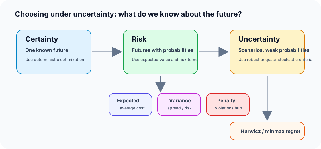
The stochasticity lecture separates three cases. Under certainty, there is one known future. Under risk, we know probabilities. Under deeper uncertainty, we may only have scenarios. The right decision criterion depends on which case we are in.

Formal definitions

Certainty:

\[ \min_{x \in X} F(x). \]

Risk with probabilities:

\[ \min_{x \in X} \mathbb{E}[F(x,\omega)]. \]

Monte Carlo approximation:

\[ \mathbb{E}[F(x,\omega)] \approx \frac{1}{N}\sum_{n=1}^{N} F(x,\omega^n). \]

Translation: if we cannot calculate the true expected cost, we average the cost over sampled futures.

Expected value-variance principle

For a cost problem:

\[ \text{score}(x)=\mathbb{E}[F(x,\omega)] + q\,\mathrm{Var}(F(x,\omega)). \]

\(q\) is the manager's risk weight. If \(q=0\), the manager only cares about average cost. If \(q\) is large, the manager strongly dislikes unstable outcomes.

Constraint-violation penalty

If uncertain demand can violate capacity, a penalty model can use:

\[ \text{penalty}(x,\omega)=p\max\{\text{load}(x,\omega)-\text{capacity},0\}. \]

Business translation: pay nothing if capacity is respected; pay a penalty for each unit of overload.

Worked example: expected value plus variance

Two delivery plans have these sampled costs:

Plan	Scenario costs	Average	Comment
A	20, 22, 24	22	stable
B	10, 20, 36	22	same average, more volatile

A risk-neutral manager is indifferent by expected value. A risk-aware manager may prefer A because it has lower variability.

3.7 Quasi-Stochastic Criteria: Hurwicz and Minmax Regret

Intuition

Sometimes probabilities are not trusted. The course introduces criteria for scenario-based thinking. These are useful when a manager can describe possible futures but cannot honestly assign probabilities.

Hurwicz criterion

For cost minimization, combine best and worst scenario outcomes:

\[ H(x)=(1-\lambda)\cdot \text{worst}(x)+\lambda\cdot \text{best}(x), \quad 0\le \lambda \le 1. \]

Translation: \(\lambda\) controls optimism. A high value puts more weight on the best case; a low value puts more weight on the worst case.

Minmax regret

Regret compares a decision with the best decision that could have been made if the scenario had been known:

\[ \text{regret}(x,s)=F(x,s)-\min_{x'\in X}F(x',s). \]

Then choose the decision with the smallest worst regret:

\[ \min_x \max_s \text{regret}(x,s). \]

Worked example: route choice without probabilities

Route	Clear traffic	Congestion
A	20	80
B	35	45

Worst-case costs: A has 80, B has 45, so a worst-case thinker chooses B.

Regret table:

Route	Clear regret	Congestion regret	Worst regret
A	0	35	35
B	15	0	15

Minmax regret also chooses B.

Common trap

Do not use Hurwicz or minmax regret when the exam gives reliable probabilities and asks for expected value. Use the criterion that matches the information given.

Chapter source note

Course basis: DDM stochasticity slides and tutorial repair-time PDF question. Textbook enrichment: Kochenderfer et al. on probability distributions, expected utility, and risk-aware decision evaluation; Powell on uncertainty modeling. Keep exam language focused on random variables, scenarios, and \(\omega_{k+1}\).

---