6. Approximate Dynamic Programming

6.1 Why ADP Exists

Intuition

ADP is what we use when exact Bellman recursion is mathematically correct but computationally impossible.

It asks:

How can we make good decisions without solving the full MDP?

Formal idea

Exact decision:

\[ x = \arg\min_{x\in X(S_k)} \left[ R(S_k,x) + V(S_k^x) \right] \]

ADP replaces a hard part with an approximation:

policy approximation
cost approximation
look-ahead approximation
value approximation

Properties

• ADP produces heuristic or approximate policies.
• Approximation is necessary for large problems.
• Good ADP exploits problem structure.
• The best ADP method depends on data, time, constraints, and interpretability needs.

6.2 Policy Classes

The DDM slides use Powell's policy-class idea.

Policy class	What it approximates	Plain idea
Policy Function Approximation (PFA)	policy directly	use a rule
Rolling Horizon Re-Optimization (RHO)	current decision problem	repeatedly optimize current model
Cost Function Approximation (CFA)	objective/constraints	add penalties, incentives, buffers
Look-ahead Models	limited future	simulate or solve a partial future
Value Function Approximation (VFA)	future value	estimate \(V(S_k^x)\)

flowchart TB
    A["Exact Bellman decision"] --> B["Approximate the policy<br/>PFA"]
    A --> C["Approximate current optimization<br/>RHO"]
    A --> D["Approximate cost/constraints<br/>CFA"]
    A --> E["Approximate future tree<br/>Look-ahead"]
    A --> F["Approximate value<br/>VFA"]

6.3 Policy Function Approximation

Intuition

A PFA is a direct rule. It does not compute a full future value. It says:

If the state looks like this, choose this action.

Formal definition

\[ \pi_\theta(S_k)=x \]

where \(\theta\) is a parameter such as a threshold or weight.

Properties

• Fast and interpretable.
• Easy to explain to managers.
• Can be tuned by simulation.
• May ignore important future consequences.

Worked example: dynamic knapsack

Rule from tutorial:

Accept item if Money / Space > 1.

Item	Money	Space	Money/Space	Decision
A	3	2	1.5	accept
B	2	3	0.67	reject
C	1	1	1.0	reject if strict > 1

Merits and disadvantages

Merit	Disadvantage
very fast	may be myopic
easy to communicate	depends on threshold
works with expert knowledge	may fail in unusual states

6.4 Rolling Horizon Re-Optimization

Intuition

RHO repeatedly solves the current optimization problem using available information.

Formal definition

\[ x = \arg\min_{x\in X(S)} R(S,x) \]

In the slides this is interpreted as:

Bellman decision with V = 0

Translation:

The method does not explicitly include future value.

Properties

• Uses standard optimization models.
• Practical for routing, scheduling, and assignment.
• Can handle constraints well.
• May consume resources too early.

Worked example: closest driver

Driver	Immediate pickup cost	Future effect
Central driver	4	leaves downtown uncovered
Outer driver	7	preserves downtown coverage

RHO chooses central driver because 4 < 7. A future-aware method may choose outer driver.

6.5 Cost Function Approximation

Intuition

CFA modifies the objective or constraints so a short-sighted model behaves more future-aware.

Formal definition

Modified objective:

\[ x = \arg\min_{x\in X(S)} \left[ R(S,x)+I(S,x) \right] \]

where:

• \(R(S,x)\) is the original cost,
• \(I(S,x)\) is an incentive or penalty.

Constraint modification:

\[ (A+\Theta)x \le b+\theta \]

Translation:

Change either the score or feasible set to discourage bad decisions.

Properties

• Often easier than modeling full uncertainty.
• Practical when managers know what behavior is bad.
• Penalties and buffers must be tuned.
• Feasibility must be checked.

Worked example: vehicle preservation

Original cost:

pickup time

Penalty:

\[ I(S,x)= \begin{cases} 6, & \text{if }x\text{ uses the last downtown driver},\\ 0, & \text{otherwise}. \end{cases} \]

Option	Pickup cost	Penalty	Modified cost
downtown driver	4	6	10
outer driver	7	0	7

CFA chooses outer driver.

Merits and disadvantages

Approach	Merits	Disadvantages
Objective penalty	easy to add to model	penalty tuning is hard
Constraint buffer	enforces safety	may be too conservative
Time-dependent penalty	adapts to state/time	more parameters to estimate

6.6 Value Function Approximation

Intuition

VFA estimates future value when exact future value is impossible.

Formal definition

Exact:

\[ x = \arg\min_{x\in X(S_k)} \left[ R(S_k,x) + V(S_k^x) \right] \]

Approximate:

\[ x = \arg\min_{x\in X(S_k)} \left[ R(S_k,x)+\hat V(S_k^x) \right] \]

Properties

• More future-aware than RHO.
• Can learn from simulation.
• Needs useful features.
• Can be wrong if the approximation is poor.

Worked example

Decision	Immediate cost	Approx future cost	Total
A	4	20	24
B	7	10	17

VFA chooses B because total cost is lower.

6.7 Look-Ahead Models

Intuition

Look-ahead builds a limited future tree or scenario model from the current state.

Formal idea

\[ \text{estimated value of }x = R(S_k,x)+\text{simulated or optimized value over a limited future}. \]

Properties

• More anticipatory than RHO.
• Computationally heavier.
• Quality depends on scenarios and horizon.
• Only the first decision is implemented.

Approach comparison

Method	Uses uncertainty?	Uses optimization?	Main weakness
Deterministic look-ahead	usually forecasts only	yes	ignores uncertainty
Stochastic look-ahead	yes, scenarios	often	expensive
Rollout	yes, simulation	base policy	base policy quality matters
MSA	yes, many scenarios	yes or repeated solves	scenario design matters

6.8 ADP Exam Template

ADP is used because exact dynamic programming is infeasible in large stochastic dynamic problems. ADP approximates parts of the Bellman decision. PFA approximates the policy directly, RHO repeatedly optimizes the current problem, CFA modifies costs or constraints, look-ahead solves a limited future, and VFA approximates future value \(V(S_k^x)\).

6.9 Choosing and Comparing ADP Methods

Intuition

ADP methods are not rivals in a tournament where one always wins. They are tools for different business situations. The exam often asks you to compare them, so answer in terms of what each method approximates.

flowchart TB
    A["Business problem too large for exact DP"]:::problem
    A --> B["Need fast transparent rule?"]:::question
    A --> C["Have strong optimization model?"]:::question
    A --> D["Know the myopic bias?"]:::question
    A --> E["Can sample future scenarios?"]:::question
    A --> F["Can learn future values?"]:::question
    B --> B1["PFA"]:::method
    C --> C1["RHO"]:::method
    D --> D1["CFA"]:::method
    E --> E1["Look-ahead / MSA / rollout"]:::method
    F --> F1["VFA"]:::method
    classDef problem fill:#fee2e2,stroke:#dc2626,stroke-width:2px,color:#0f172a;
    classDef question fill:#e0f2fe,stroke:#0284c7,stroke-width:2px,color:#0f172a;
    classDef method fill:#dcfce7,stroke:#16a34a,stroke-width:2px,color:#0f172a;

Detailed comparison

Method	What it approximates	Best business use	Main drawback
PFA	policy directly	fast operational rule	can ignore future value
RHO	current optimization	strong static solver exists	often myopic
CFA	cost/constraints	known bias needs correction	parameters hard to tune
Look-ahead	limited future	future scenarios matter	computationally expensive
VFA	future value	repeated simulation/data available	needs features and validation

Worked example: same-day delivery method choice

Problem:

Many orders arrive during the day.
Vehicles have capacity and time windows.
Future demand is uncertain.

Possible design:

RHO solves the current routing problem.
CFA penalizes using the last vehicle in a high-demand zone.
Look-ahead samples future orders during peak periods.
VFA estimates the value of remaining vehicle capacity by zone and time.

Exam insight:

Combined ADP is often more realistic than choosing exactly one class.

6.10 Course Policy-Class Map and Method Choice

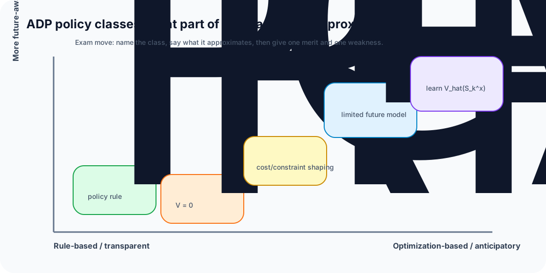
Mental model

The ADP lecture is organized around a practical question: which part of the impossible Bellman equation should we approximate? Each policy class answers that differently.

Class	Bellman part approximated	Course-style example	What to say in the exam
PFA	direct mapping \(S_k\to x\)	knapsack threshold or Trucks & Barges rules	fast and interpretable, but may miss future value
RHO	solves current deterministic problem	current routing/assignment	uses optimization, but \(V=0\) so it is myopic
CFA	modifies reward/constraints	reserve capacity, penalize using scarce drivers	practical bias correction, but tuning is hard
Look-ahead	limited future tree/model	MSA for future orders	anticipatory, but computationally expensive
VFA	approximate \(V(S_k^x)\)	lookup table for time/capacity	learns future value, but needs features and validation

6.11 Tutorial Example: Dynamic Knapsack Across Policy Classes

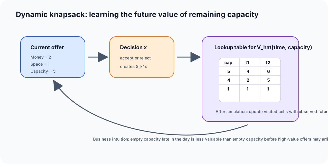
Problem setup

A knapsack has limited capacity. At each decision point, offers appear with money and space. Accepting earns money but consumes capacity that might be needed later.

PFA version

\[ \pi_\theta(S_k)=\text{accept if }\frac{\text{money}}{\text{space}}>\theta. \]

If \(\theta=1\), accept offers earning more than 1 money per unit of capacity.

CFA version

Add a penalty for using scarce capacity early:

\[ \min_x \left[-\text{money}(x)+I(S_k,x)\right]. \]

Example penalty: reserve 6 units for three remaining periods, so early low-density offers become unattractive.

Look-ahead / MSA version

Sample possible future offers, solve a combined current-plus-future knapsack for each scenario, and implement only the current accept/reject decision that performs best across scenarios.

VFA version

Use a lookup table:

\[ \hat V(t,b) \approx \text{future value of having capacity } b \text{ at time } t. \]

Decision rule:

\[ \max_{x\in X(S_k)} \left[\text{money}(x)+\hat V(t+1,b^x)\right]. \]

Business translation: the model accepts an item only if its money plus the value of the remaining capacity is better than rejecting it.

Chapter source note

Course basis: DDM ADP policy-class slides, RHO/CFA/VFA/look-ahead slides and tutorials. Textbook enrichment: Powell on policy classes, cost function approximations, and direct lookahead; Kochenderfer et al. on approximate value functions and online planning. Course notation remains primary.

---