2. Information Modeling and Decision Making

2.1 Information Model vs Decision Model

Intuition

An information model describes what is known or predicted. A decision model describes what can be done.

Information model questions:

What demand might appear?
How long might travel take?
Which resources are available?
What probabilities or forecasts describe uncertainty?

Decision model questions:

Which action is feasible?
What constraints apply?
What cost or reward is produced?
Which objective should be optimized?

Formal definition

Information model components often define:

\[ S_k,\qquad \omega_{k+1},\qquad P \]

Decision model components often define:

\[ X(S_k),\qquad R(S_k,x),\qquad \text{constraints},\qquad \text{objective},\qquad \pi \]

Translation:

The information model describes the world. The decision model chooses actions in that world.

Properties

• Forecasts are information, not decisions.
• Optimization constraints are decision-model elements.
• Information quality affects decision quality.
• More detailed information can improve decisions but can also make optimization harder.

flowchart LR
    A["Historical data"] --> B["Information model"]
    C["Real-time observations"] --> B
    D["Forecasts and probabilities"] --> B
    B --> E["State S_k and new information omega"]
    E --> F["Decision model"]
    G["Feasible actions X(S_k)"] --> F
    H["Objective R(S_k,x)"] --> F
    F --> I["Decision x"]

Worked example: ride-hailing

Information model:

Category	Examples
Environment	traffic lights, traffic jams, travel times, occupied charging stations
Resources	fleet size, vehicle types, capacities, battery status
Demand	pickup, destination, request time, passenger count, accessibility needs

Decision model:

• Decision points: each request or every few minutes.
• State \(S_k\): time, vehicle locations, open requests, traffic conditions.
• Decision \(x\): accept/reject, assign vehicle, reposition idle vehicle.
• Reward/cost \(R(S_k,x)\): revenue - pickup delay - travel cost - service penalty.
• Objective: maximize expected profit or service quality.

Exam phrase

The information model provides decision-relevant data, predictions, probabilities, and scenarios. The decision model uses this information to define feasible decisions, constraints, rewards or costs, and the objective.

2.2 Utility, Cost, and Expected Performance

Intuition

Business decisions often compare options using money, time, service level, or penalties. Mathematical decision making compresses these into a reward, cost, or utility.

If higher is better, call it reward or utility. If lower is better, call it cost.

Formal definition

For a deterministic decision:

\[ x=\arg\max_{x\in X(S)} R(S,x) \]

or:

\[ x=\arg\min_{x\in X(S)} C(S,x) \]

For uncertain outcomes:

\[ x = \arg\max_{x\in X(S)} E\left[R(S,x,\omega)\right] \]

or:

\[ x = \arg\min_{x\in X(S)} E\left[C(S,x,\omega)\right] \]

Here:

• \(x\) is the decision,
• \(\omega\) is random future information,
• \(E[\cdot]\) means probability-weighted average.

Properties

• Expected performance averages across possible futures.
• A risk-neutral decision maker focuses on expected value.
• A risk-averse decision maker may also care about variability and worst cases.
• Utility can combine several business goals, such as profit, delay, reliability, and fairness.

Worked example: expected utility

Two delivery options:

Option	Probability	Cost
A: normal traffic	0.8	20
A: heavy traffic	0.2	80
B: stable route	1.0	35

Expected cost of A:

\[ \begin{aligned} E[C_A] &= 0.8\cdot20 + 0.2\cdot80 \\ &= 16+16 \\ &= 32 \end{aligned} \]

Expected cost of B:

\[ \begin{aligned} E[C_B] &= 1.0\cdot35 \\ &= 35 \end{aligned} \]

Expected-cost decision:

choose A

Risk-aware interpretation:

B may still be preferred if late deliveries are very damaging.

2.3 The Five-Component Sequential Decision Model

Intuition

Powell's framework is useful because it makes every sequential decision problem look like the same basic machine:

1. state,
2. decision,
3. exogenous information,
4. transition,
5. objective.

This matches the DDM course closely.

Formal definition in DDM notation

Component	Course notation	Plain meaning
state	\(S_k\)	what is known at decision point \(k\)
decision	\(x\in X(S_k)\)	what the decision maker can choose
exogenous information	\(\omega_{k+1}\)	new information revealed after the decision
transition	\(S_{k+1}=S^M(S_k,x,\omega_{k+1})\)	how the system moves to the next state
objective	\(\min\) or \(\max\) expected total reward/cost	what the policy tries to optimize

Properties

• This model works for logistics, inventory, pricing, routing, and service systems.
• It forces you to identify what happens before and after the decision.
• It separates decision-controlled changes from random changes.

Worked example: Trucks & Barges

State:

current day, containers in yard, destinations, due dates, known future containers

Decision:

ship by truck, barge, train, or hold in yard

Exogenous information:

random new arrivals, final clean-up costs

Transition:

tomorrow's yard = today's yard - shipped containers + new arrivals

Objective:

minimize expected transport, setup, delay, and clean-up costs

2.4 Modeling Checklist

Use this whenever asked to "model" a problem:

1. Objective.
2. Stakeholders.
3. Resources.
4. Demand.
5. Environment.
6. Decision points.
7. State \(S_k\).
8. Feasible decisions \(X(S_k)\).
9. Reward/cost \(R(S_k,x)\).
10. Stochastic information \(\omega_{k+1}\).
11. Transition.
12. Policy \(\pi\).

Common mistakes

• Forgetting stakeholders and objective.
• Naming demand but not resources.
• Describing the data but not the decision.
• Ignoring feasibility constraints.
• Treating unknown future demand as known state information.

2.5 Expected Utility and Value of Information

Intuition

Information is useful only when it can change a decision. A weather forecast, traffic forecast, or demand forecast has business value if it helps the decision maker choose a better action.

Formal definition

For reward maximization:

Value of information =
expected reward with information - expected reward without information

For cost minimization:

Value of information =
expected cost without information - expected cost with information

Translation:

Information is valuable when it improves expected business performance.

flowchart TB
    subgraph NoInfo["Without extra information"]
        A["Use average forecast"]:::info --> B["Choose one decision"]:::decision --> C["Expected cost"]:::cost
    end
    subgraph WithInfo["With extra information"]
        D["Observe signal<br/>traffic/weather/demand"]:::info --> E["Choose state-specific decision"]:::decision --> F["Lower expected cost"]:::good
    end
    C --> G["Value of information<br/>cost without info - cost with info"]:::value
    F --> G
    classDef info fill:#e0f2fe,stroke:#0284c7,stroke-width:2px,color:#0f172a;
    classDef decision fill:#ffedd5,stroke:#f97316,stroke-width:2px,color:#0f172a;
    classDef cost fill:#fee2e2,stroke:#ef4444,stroke-width:2px,color:#0f172a;
    classDef good fill:#dcfce7,stroke:#16a34a,stroke-width:2px,color:#0f172a;
    classDef value fill:#f5f3ff,stroke:#7c3aed,stroke-width:2px,color:#0f172a;

Worked example: route decision with traffic forecast

Without a traffic forecast:

Expected cost of Route A = 30
Expected cost of Route B = 34
Choose Route A.
Expected cost = 30

With a forecast:

Forecast	Probability	Best route	Cost
clear roads	0.6	A	20
congestion	0.4	B	28

Expected cost with information:

\[ 0.6\cdot20 + 0.4\cdot28 = 12+11.2=23.2 \]

Value of information:

\[ 30-23.2=6.8 \]

Business interpretation:

The forecast is worth up to 6.8 cost units per decision because it allows the firm to adapt route choice.

Approach comparison

Information approach	Merit	Disadvantage	Use when
Historical average	simple and stable	misses context	low variability settings
Conditional forecast	adapts to state	needs data/features	demand/travel depends on context
Scenario forecast	captures several futures	more computation	decisions are sensitive to uncertainty
Real-time signal	highly adaptive	may be noisy or costly	decisions can still react

2.8 Slide Case: Time-Dependent Travel-Time Information Model

Mental model

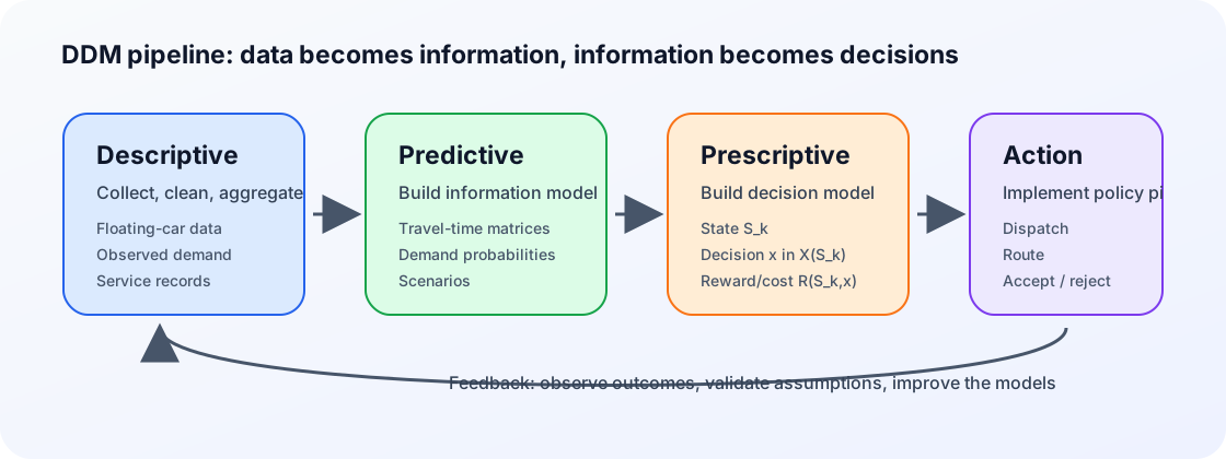
The travel-time case in the slides is a perfect example of why information modeling is work. The raw data does not arrive as a neat travel-time matrix. It arrives as vehicle positions, timestamps, street segments, speeds, outliers, missing observations, and uneven spatial coverage. The information model is the bridge from this messy data to a decision model a routing algorithm can use.

Formal representation

Let \(\tau_{ij}(t)\) be the travel time from location \(i\) to location \(j\) if the vehicle starts at time \(t\).

A static model uses:

\[ \tau_{ij}. \]

A time-dependent model uses:

\[ \tau_{ij}(t). \]

Translation: the travel time between the same two customers can be different at 8:00, 12:00, and 17:00.

Properties from the slides

• Floating-car data can be used to estimate speeds and travel times.
• Some road segments have many observations; others have few.
• Aggregation turns millions of observations into usable matrices.
• Normalization and clustering help reveal recurring traffic patterns.
• Spatial and temporal validation check whether clusters make business sense.
• A more realistic information model often forces a more complex decision model.

Worked example: why a route changes by start time

Suppose a driver must visit customers A, B, and C.

Start time	Downtown travel	Outer-road travel	Sensible first area
7:30	slow	normal	outskirts first
12:00	normal	normal	nearest / cheapest insertion
17:00	very slow	normal	avoid downtown first

A static model may produce one route for all start times. A time-dependent model may produce different sequences because the cost of visiting downtown changes over the day.

Exam phrasing

A strong answer says: the information model provides time-dependent travel times \(\tau_{ij}(t)\), possibly obtained by aggregation and clustering of observed vehicle data. The decision model then uses these time-dependent values when defining feasible routes and calculating the objective.

2.9 Course Distinction: Model Detail Is Not Automatically Better

Intuition

The slides repeatedly show the same trade-off: more detailed information can improve decision quality, but it also increases model complexity. A business analyst should not simply ask for the most detailed model. They should ask whether the extra detail changes decisions enough to justify the extra complexity.

Formal idea

A richer information model changes either the state or transition model:

\[ S_k = (\text{resources}, \text{demand}, \text{environment}). \]

Adding time-dependent traffic means the environment component may include the current time and a travel-time matrix:

\[ S_k = (t_k, \text{vehicle positions}, \text{open orders}, \tau(t_k)). \]

Worked example: two information models

Model	Information	Decision consequence
Static travel time	one average matrix	route can be planned once
Time-dependent travel time	matrix changes by time	route sequence and path may change during the day
Stochastic travel time	probability distribution or scenarios	decision should consider risk and expected future cost

Common trap

Do not call a forecast a decision. A forecast of demand is information. Accepting, rejecting, assigning, routing, or repositioning is a decision.

Chapter source note

Course basis: DDM slides/tutorials on information models, decision models, and ride-hailing environment/resources/demand. Textbook enrichment: Kochenderfer et al. on expected utility and value of information; Powell on the five-component sequential decision model. In the exam, express the final model using \(S_k\), \(X(S_k)\), \(R(S_k,x)\), \(\omega_{k+1}\), and \(\pi\).

---