1. Overview

1.1 What Dynamic Decision Making Is

Intuition

Dynamic Decision Making (DDM) studies decisions that happen repeatedly over time. The decision maker does not simply create one plan and follow it blindly. Instead, the decision maker observes the current situation, acts, receives new information, and acts again.

Examples:

• a delivery platform assigns drivers as orders arrive,
• a ride-hailing platform decides whether to accept and assign requests,
• a logistics company ships containers by truck, barge, train, or storage each day,
• an inventory manager orders stock before demand is known,
• a repair company schedules technicians when repair times are uncertain.

The key idea is that today's decision changes tomorrow's options. Sending the closest driver might be good now but bad later if it leaves a high-demand area uncovered.

Formal definition

A dynamic decision problem has:

Object	Course notation	Meaning
decision points	\(k=0,1,\ldots,K\)	times when decisions are made
state	\(S_k\)	decision-relevant information at decision point \(k\)
feasible decision	\(x\in X(S_k)\)	an action allowed in state \(S_k\)
reward/cost	\(R(S_k,x)\)	immediate business impact of decision \(x\)
next state	\(S_{k+1}\)	the next decision situation
policy	\(\pi\)	rule or method for choosing decisions

A policy is:

\[ \pi(S_k)=\text{decision chosen in state }S_k \]

Translation:

A policy is a decision rule. It tells us what to do for each possible situation.

Properties

• The solution is a policy, not just a fixed plan.
• Good decisions account for future consequences.
• The model must specify what is known before the decision and what is revealed after it.
• If future information is uncertain, the objective is usually expected total reward or cost.

Worked example: ride-hailing

At 8:00 AM, a car is downtown and a customer appears nearby. Accepting the customer gives immediate revenue. But the car may then leave downtown just before a high-demand wave.

State:

\[ S_k = (\text{current time},\ \text{car locations},\ \text{request details}, \ \text{traffic},\ \text{expected demand}) \]

Decision:

\[ x\in\{\text{accept and assign},\ \text{reject},\ \text{wait}\} \]

Cost/reward:

\[ R(S_k,x)=\text{revenue}-\text{pickup delay}-\text{operating cost} \]

Future consequence:

\[ S_k^x = \text{car distribution after assignment} \]

Business lesson:

The best current assignment is not always the best dynamic policy.

Exam phrase

The problem is dynamic because decisions are made at multiple decision points and new information arrives between decisions. The solution should be a policy that maps each state \(S_k\) to a feasible decision \(x\in X(S_k)\), rather than a single fixed plan.

1.2 Static, Stochastic, Dynamic, and Adaptive

Intuition

These words are easy to mix up:

• Static means one decision or one plan.
• Dynamic means several connected decisions.
• Deterministic means future effects are known.
• Stochastic means future effects are uncertain.
• Adaptive means the decision maker reacts to new information.

You can have a dynamic deterministic problem: many decisions over time, but all future information is known. You can also have a static stochastic problem: one decision today before uncertain demand, with no later reaction.

Formal classification

Type	Decisions over time?	Uncertainty?	Example
Static deterministic	no	no	fixed TSP with known travel times
Static stochastic	no	yes	order inventory once before random demand
Dynamic deterministic	yes	no	known production schedule over days
Dynamic stochastic	yes	yes	delivery with random future orders

Properties

• Dynamism is about timing and reaction.
• Stochasticity is about uncertainty.
• Adaptivity requires later decisions after new information.

Worked example: inventory

Static stochastic:

Choose order quantity today.
Demand tomorrow is random.
No second chance.

Dynamic stochastic:

Choose order quantity today.
Observe demand.
Update inventory.
Order again tomorrow.

Common mistake

Do not write:

The problem is dynamic because travel times are uncertain.

Better:

Travel-time uncertainty makes the problem stochastic. The problem is dynamic if the decision maker can adapt decisions later as new travel-time information or requests arrive.

1.3 Course Roadmap

Intuition

The course builds from simple ideas to more advanced decision policies:

1. Understand the problem.
2. Separate information from decisions.
3. Model uncertainty.
4. Model decisions over time.
5. Combine uncertainty and dynamism in MDPs.
6. Use ADP when exact recursion is too large.
7. Use sampling to approximate uncertain futures.
8. Use supervised learning to build information models.
9. Use reinforcement learning ideas to learn values and policies.
10. Combine methods for practical decision support.

flowchart TB
    A["Overview"] --> B["Information models"]
    B --> C["Stochasticity"]
    C --> D["Dynamism"]
    D --> E["Stochastic dynamic decision problems"]
    E --> F["Approximate dynamic programming"]
    F --> G["Sampling methods"]
    G --> H["Supervised learning"]
    H --> I["Reinforcement learning"]
    I --> J["Combined methods"]
    J --> K["Exam preparation"]

Exam phrase

DDM combines information modeling, decision modeling, uncertainty, and sequential decisions. The central challenge is to design a policy that performs well over time when future information is uncertain.

1.4 Mental Model: The Business Clock

Intuition

Think of a dynamic decision problem as a business clock. At every tick, the firm asks three questions:

What do we know now?
What can we do now?
What future situation will this create?

The first question is the state \(S_k\). The second question is the feasible decision set \(X(S_k)\). The third question is the future value of the post-decision state \(S_k^x\).

flowchart LR
    subgraph Now["Now: decision point k"]
        S["State S_k<br/>what the business knows"]:::state
        X["Feasible decisions<br/>x in X(S_k)"]:::decision
        R["Immediate result<br/>R(S_k,x)"]:::reward
    end
    subgraph Bridge["Bridge to the future"]
        PX["Post-decision state<br/>S_k^x"]:::post
        W["New information<br/>omega_{k+1}"]:::random
    end
    subgraph Later["Later: decision point k+1"]
        SN["Next state<br/>S_{k+1}"]:::state
        PI["Policy reacts again<br/>pi(S_{k+1})"]:::policy
    end
    S --> X --> R
    X --> PX --> W --> SN --> PI
    classDef state fill:#e8f3ff,stroke:#2563eb,stroke-width:2px,color:#0f172a;
    classDef decision fill:#fff7ed,stroke:#ea580c,stroke-width:2px,color:#0f172a;
    classDef reward fill:#ecfdf5,stroke:#059669,stroke-width:2px,color:#0f172a;
    classDef post fill:#f5f3ff,stroke:#7c3aed,stroke-width:2px,color:#0f172a;
    classDef random fill:#fef2f2,stroke:#dc2626,stroke-width:2px,color:#0f172a;
    classDef policy fill:#f8fafc,stroke:#475569,stroke-width:2px,color:#0f172a;

Worked example: delivery slot acceptance

An e-grocery company can accept one more delivery order for tonight.

Immediate view:

\[ \begin{aligned} \text{revenue from accepting} &= 12 \\ \text{extra route cost} &= 5 \\ \text{immediate reward} &= 12-5=7 \end{aligned} \]

Dynamic view:

Accepting uses scarce evening capacity.
If a high-value order arrives later, the company may have to reject it.

Decision now	Immediate reward	Future value	Total
Accept current order	7	10	17
Reject current order	0	25	25

Dynamic decision:

Reject current order if preserving capacity has enough future value.

1.7 Course-Enriched Roadmap: What The Slides Are Really Building Toward

Mental model

The slide deck starts with a business problem, not a formula. A company observes a messy real-world system, turns observations into an information model, turns the information model into a decision model, and then needs methods because uncertainty and dynamism make the exact problem too large.

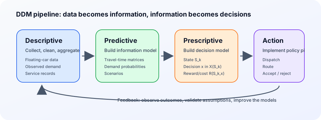
Formal course framing

A dynamic decision problem is built around repeated decisions:

\[ S_k \rightarrow x \in X(S_k) \rightarrow S_k^x \rightarrow \omega_{k+1} \rightarrow S_{k+1}. \]

Business translation: before each decision, the manager observes the state; the decision changes the controllable part of the system; then new information arrives from the world.

Worked example: from static routing to DDM

A parcel company first builds a static route for the whole day. That is a plan. But if travel times change, orders arrive, or drivers get delayed, the company needs a policy:

Stage	Business question	DDM object
Observe	Where are drivers and orders now?	\(S_k\)
Decide	Who should go where?	\(x\in X(S_k)\)
Commit	What changed because of the decision?	\(S_k^x\)
Learn	What new demand/travel time appeared?	\(\omega_{k+1}\)
Repeat	What is the next decision situation?	\(S_{k+1}\)

Common trap

Do not start an exam answer with algorithms. Start with the problem model. Most DDM marks come from naming the state, decisions, uncertainty, transitions, and objective clearly.

Chapter source note

Course basis: DDM overview slides on information/decision modeling, stochasticity, dynamism, and ADP motivation. Textbook enrichment: Kochenderfer et al. on decision making under uncertainty and Powell on sequential decision problems and policies. Use DDM notation in exam answers.

---