5. Stochastic and Dynamic Decision Problems
5.1 Markov Decision Processes
Intuition
An MDP is the course's formal container for stochastic dynamic decision problems. It says:
If I know the current state and choose a decision, I can describe immediate reward/cost and possible next states.
The state should summarize everything decision-relevant. You do not need the whole history if the state contains what matters for future decisions.
Formal definition
An MDP has:
| Component | Notation | Meaning |
|---|---|---|
| state | \(S_k\in\mathcal{S}\) | information available before decision \(k\) |
| decision | \(x\in X(S_k)\) | feasible action in state \(S_k\) |
| reward/cost | \(R(S_k,x)\) | immediate business impact |
| post-decision state | \(S_k^x\) | state after decision, before new randomness |
| stochastic information | \(\omega_{k+1}\) | new information revealed after the decision |
| transition probabilities | \(P:\mathcal{S}\times X\times\mathcal{S}\rightarrow[0,1]\) | probabilities of next states |
| horizon | \(k=0,1,\ldots,K\) | decision points in the problem |
Transition probability:
Translation:
Properties
- States must be decision-relevant, not necessarily exhaustive.
- Feasible decisions depend on the state.
- Rewards/costs are immediate.
- Future consequences are represented through post-decision states and transitions.
flowchart LR
    A["Decision state S_k"] --> B["Decision x"]
    B --> C["Reward/cost R(S_k,x)"]
    B --> D["Post-decision state S_k^x"]
    D --> E["Transition probabilities P"]
    E --> F["Next state S_{k+1}"]
Worked example: pizza delivery MDP
Decision points:
State:
Decision:
Cost:
Post-decision state:
Stochastic information:
Objective:
5.2 Bellman Equation
Intuition
The Bellman idea is "now plus later":
It prevents purely myopic decisions.
Formal definition
Reward maximization:
Cost minimization:
Post-decision value:
Translation:
flowchart TB
    A["Current state S_k"] --> B1["Decision A"]
    A --> B2["Decision B"]
    B1 --> C1["Immediate R + future V"]
    B2 --> C2["Immediate R + future V"]
    C1 --> D["Choose best total"]
    C2 --> D
Worked example: accepting a request
Reward maximization:
| Decision | Immediate reward | Future value | Total |
|---|---|---|---|
| Accept | 20 | 40 | 60 |
| Reject | 0 | 70 | 70 |
Decision:
Interpretation:
5.3 Exact Dynamic Programming
Intuition
Exact dynamic programming solves an MDP by working backward from the end. It is powerful for small problems and impossible for many real ones.
Formal backward calculation
Terminal value:
Backward step:
Properties
- Exact if the full MDP is known and small.
- Requires enumerating states, decisions, and transitions.
- Gives a benchmark for small exam graphs.
- Breaks down under dimensionality.
Worked example: small minimization
Decision A:
Decision B:
Choose B because:
5.4 Curses of Dimensionality
Intuition
The curse of dimensionality means that exact recursion grows too large.
The course emphasizes three spaces:
Formal explanation
Exact DP must evaluate:
If each part grows, total calculations can grow explosively.
Properties
- More resources create more states.
- More customers create more decisions.
- More random future outcomes create more transitions.
- Continuous time and locations make the problem harder.
flowchart LR
    A["More customers"] --> D["More states and decisions"]
    B["More vehicles"] --> D
    C["More random futures"] --> E["More transitions"]
    D --> F["Exact DP infeasible"]
    E --> F
    F --> G["Need ADP"]
Worked example
Small classroom MDP:
Real delivery system:
Conclusion:
5.5 Exam Template
An MDP model should define decision points, state \(S_k\), feasible decisions \(x\in X(S_k)\), immediate reward/cost \(R(S_k,x)\), post-decision state \(S_k^x\), stochastic information \(\omega_{k+1}\), transition probabilities \(P\), and the objective. Exact dynamic programming evaluates immediate reward/cost plus future value, but for realistic problems the state, decision, and information spaces become too large, motivating ADP.
5.6 Bellman as a Business Balance Sheet
Intuition
The Bellman equation is easiest to understand as a balance sheet for a decision. Every decision has:
A manager might be tempted to look only at current impact. DDM forces the manager to put the future impact on the same line.
flowchart TB
    S["State S_k"]:::state --> D1["Decision A"]:::decision
    S --> D2["Decision B"]:::decision
    D1 --> A1["Immediate<br/>R(S_k,A)"]:::now
    D1 --> A2["Future<br/>V(S_k^A)"]:::future
    D2 --> B1["Immediate<br/>R(S_k,B)"]:::now
    D2 --> B2["Future<br/>V(S_k^B)"]:::future
    A1 --> TA["Total A"]:::total
    A2 --> TA
    B1 --> TB["Total B"]:::total
    B2 --> TB
    TA --> C["Choose best total"]:::choice
    TB --> C
    classDef state fill:#e0f2fe,stroke:#0284c7,stroke-width:2px,color:#0f172a;
    classDef decision fill:#ffedd5,stroke:#f97316,stroke-width:2px,color:#0f172a;
    classDef now fill:#dcfce7,stroke:#16a34a,stroke-width:2px,color:#0f172a;
    classDef future fill:#ede9fe,stroke:#7c3aed,stroke-width:2px,color:#0f172a;
    classDef total fill:#fef9c3,stroke:#ca8a04,stroke-width:2px,color:#0f172a;
    classDef choice fill:#f8fafc,stroke:#334155,stroke-width:2px,color:#0f172a;
Worked example: inventory with terminal penalty
An inventory manager decides whether to order \(x=0\) or \(x=5\) units before the final day. Ordering costs 2 per unit. If inventory is short at the end, shortage penalty is 8 per missing unit.
Current inventory:
Demand tomorrow has two possibilities:
| Demand | Probability |
|---|---|
| 4 | 0.5 |
| 8 | 0.5 |
Decision \(x=0\):
Decision \(x=5\):
Decision:
Order 5 units because \(10<24\).
5.7 Slide Worked Example: Parcel Replenishment Recursion
Mental model
The MDP recursion example in the slides is about a vehicle with limited fill level serving customers. After serving a customer, demand can be low or high. The vehicle may choose to go directly to the next customer or replenish at the depot. This is a small classroom version of a huge real routing problem.
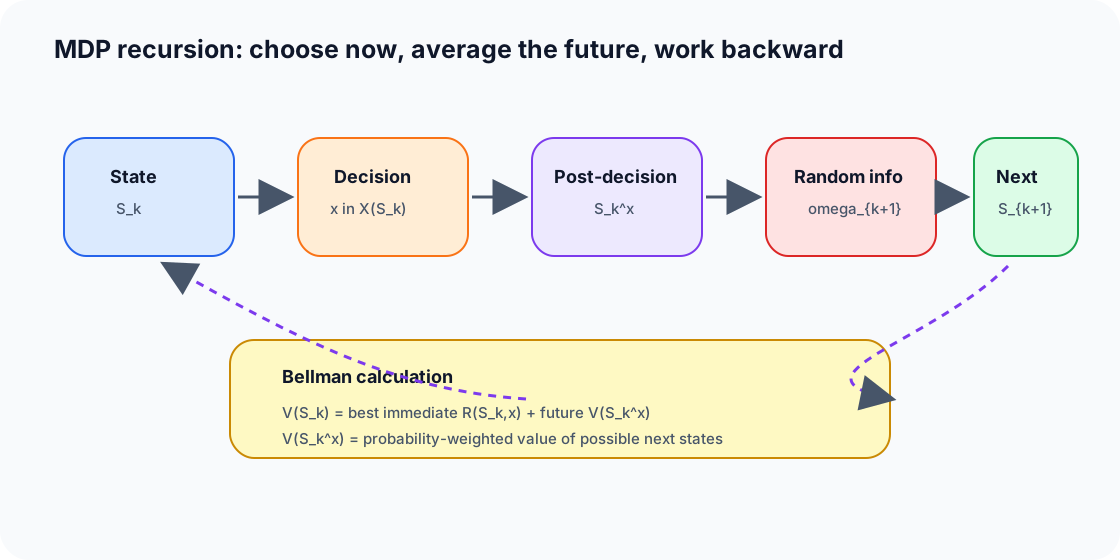
Course components
| Component | Example content |
|---|---|
| Decision point \(k\) | before visiting the next customer |
| State \(S_k\) | current position and fill level |
| Decision \(x\) | go next (\(N\)) or replenish at depot (\(A\)) |
| Reward/cost \(R(S_k,x)\) | travel time or penalty |
| Post-decision state \(S_k^x\) | position/fill after the chosen action before demand is realized |
| \(\omega_{k+1}\) | customer demand realization |
| Transition | updated position and fill level |
Formal Bellman calculation
For minimization:
If demand has two equally likely outcomes after \(S_k^x\), then:
Small numeric version
Suppose state \(S_k=(\text{position }1,\text{ fill }2)\).
| Decision | Immediate travel cost | Possible next values | Expected future value | Total |
|---|---|---|---|---|
| N | 15 | 40, 40 | 40 | 55 |
| A | 20 | 27, 27 | 27 | 47 |
Decision:
Business interpretation: replenishing costs more immediately, but it protects the future enough to be better overall.
5.8 Slide Numbers: Why Exact DP Breaks
The course example is intentionally tiny, yet already has many objects:
| Object | Count in slide example |
|---|---|
| Decision points | 4 |
| States | 12 |
| Decisions | 17 |
| Post-decision states | 12 |
| Transitions | 16 |
| Calculations | 16 |
When the dimensions increase, the slide deck shows explosive growth: more demand options can create hundreds of states, more customers can create hundreds of thousands of states, and adding routing decisions can push the count into billions.
Exam translation
The curse of dimensionality is not only about many states. It also includes the decision space and the information/transition space. Exact recursion must handle all three.
Chapter source note
Course basis: DDM MDP slides, Bellman/value-function slides, tutorial MDP graph calculations. Textbook enrichment: Kochenderfer et al. on MDPs, value functions, and exact solution methods; Powell on the universal sequential-decision model. Use DDM post-decision notation in the exam.